Anomaly Detection at Scale: What a Clean Benchmark Can’t Tell You

Case study — one-class kernel machines on 2M+ ride-hail trips, developed on proprietary regulator data and replicated end-to-end on public NYC-TLC data.

The problem

British Columbia’s taxi and ride-hail operators are required to submit trip-level records — GPS coordinates, fares, distances, durations — to the BC Ministry of Transportation and Transit’s Passenger Transportation Data Warehouse. That data feeds licensing and policy decisions for the sector, so its quality matters — and quality has been a challenge since the warehouse launched. The regulator’s defence is rule-based validation: eight business rules checking that fares, distances, and durations each fall within a plausible range.

Rules have a structural blind spot: they check features one at a time. A $330 fare passes the fare rule; an 11 km distance passes the distance rule; a $330 fare for an 11 km trip is flagged by nothing. The same holds for a 143 km trip “completed” in 5 minutes, or pickup and dropoff coordinates recorded in opposite hemispheres. The anomalies that matter live in the relationships between features — exactly where a rule system can’t see. Catching them is a one-class problem: you can characterize normal trips from the rule-compliant population, but the anomalies arrive in shapes nobody enumerated in advance.

The scale is the second half of the problem. A One-Class Restricted Kernel Machine learns that inlier distribution in kernel space, but exact kernel methods don’t survive contact with 2M rows — the kernel matrix alone is terabytes. I used Nyström landmark approximation: represent the kernel space through a few thousand well-chosen landmark trips instead of all of them, cutting training from intractable to seconds. Every example above is real, drawn from a post-hoc cohort of 806 trips the model flagged that pass all eight rules — four distinct failure types, independently confirmed by IsolationForest.

What I found

Seventeen logged experiment iterations on the BC data, then a six-iteration replication on public data. Four results carry the story:

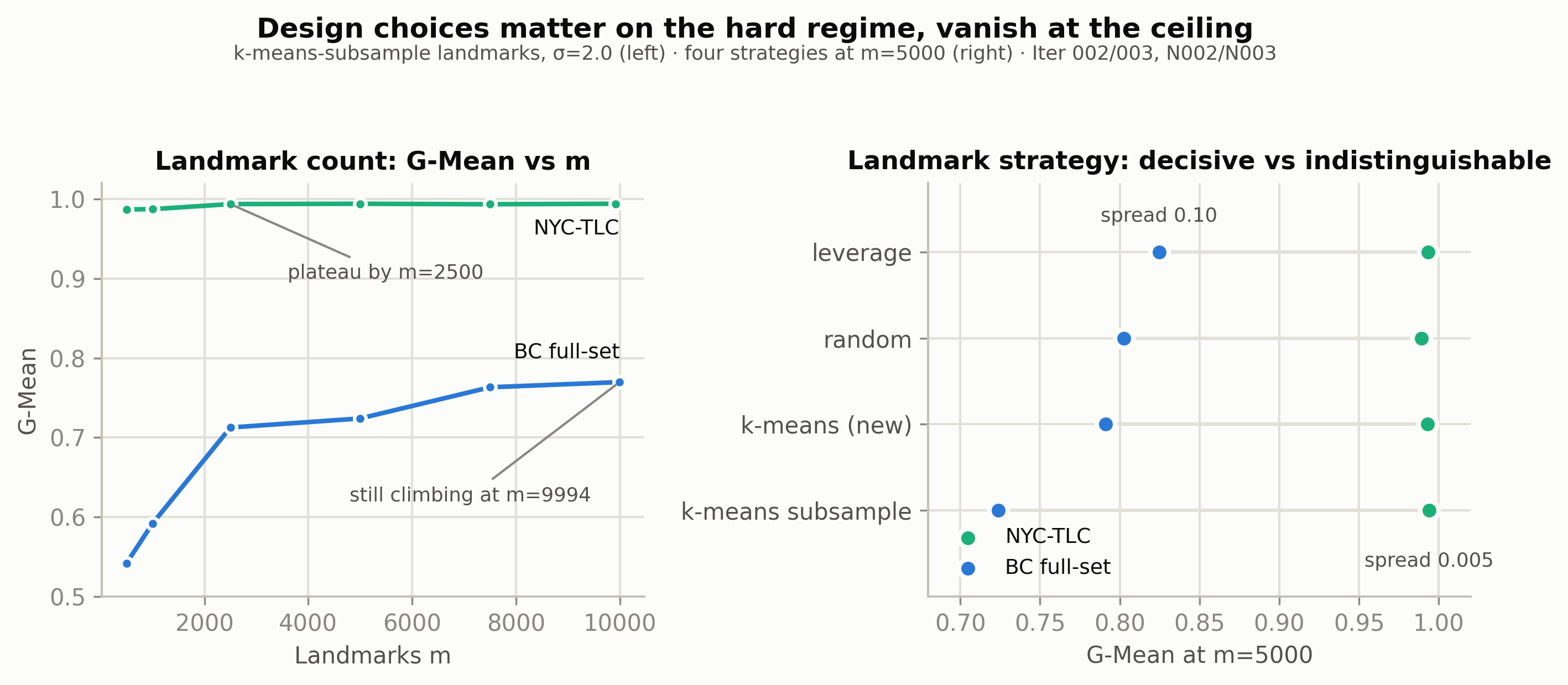
1. Which landmarks you pick beats how many you pick. Approximate-leverage landmark selection at m=5,000 outperformed the baseline k-means selection at m=9,994 on both G-Mean and ROC-AUC — at 42% of the runtime. The default choice (subsample k-means centroids) was the weakest of four strategies tested.

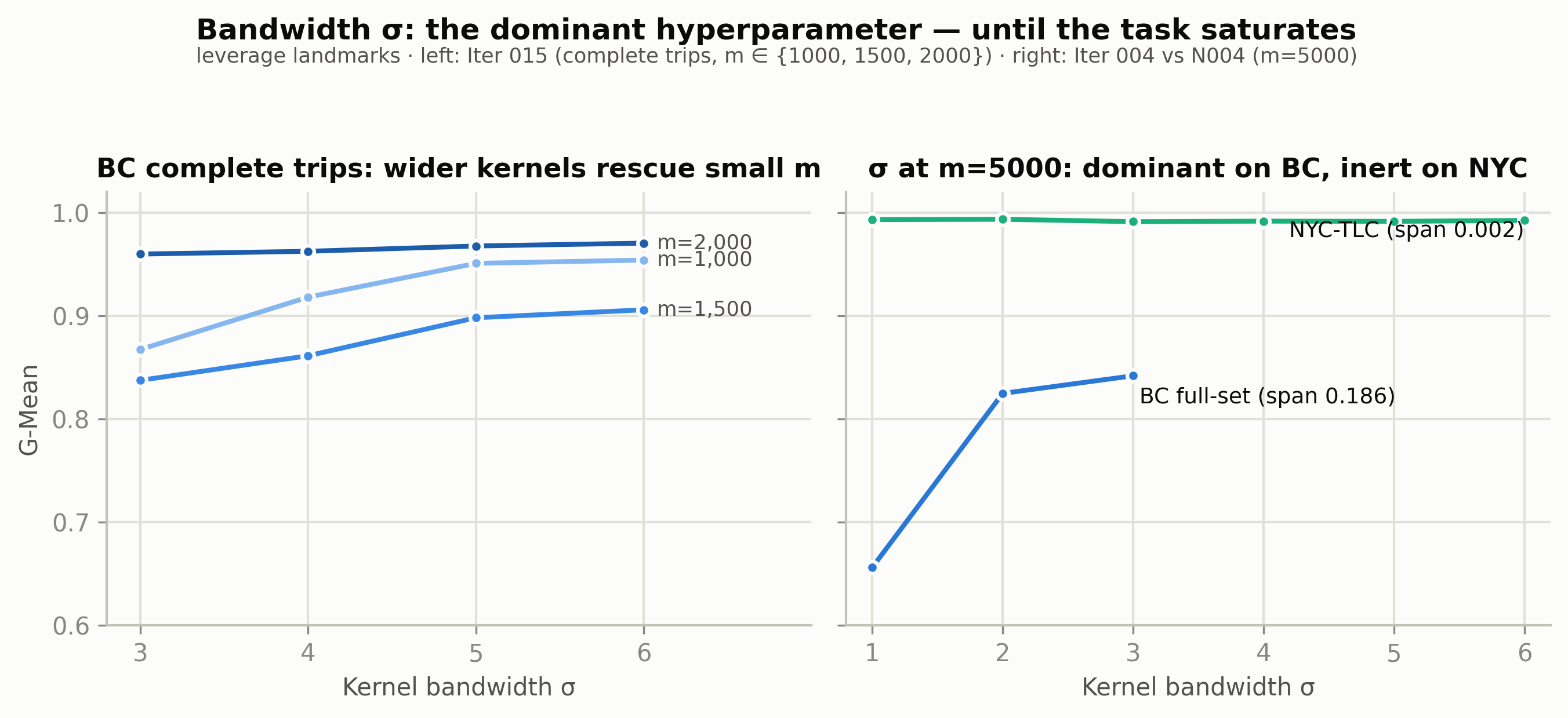
2. Kernel bandwidth is the only hyperparameter that matters here. σ moved G-Mean by 0.19 across its range; the learning rate η was inert everywhere it was tested. Wider kernels also rescue small landmark budgets — m=1,000 with σ=6 nearly matches m=2,500 with σ=3 at a third of the cost.

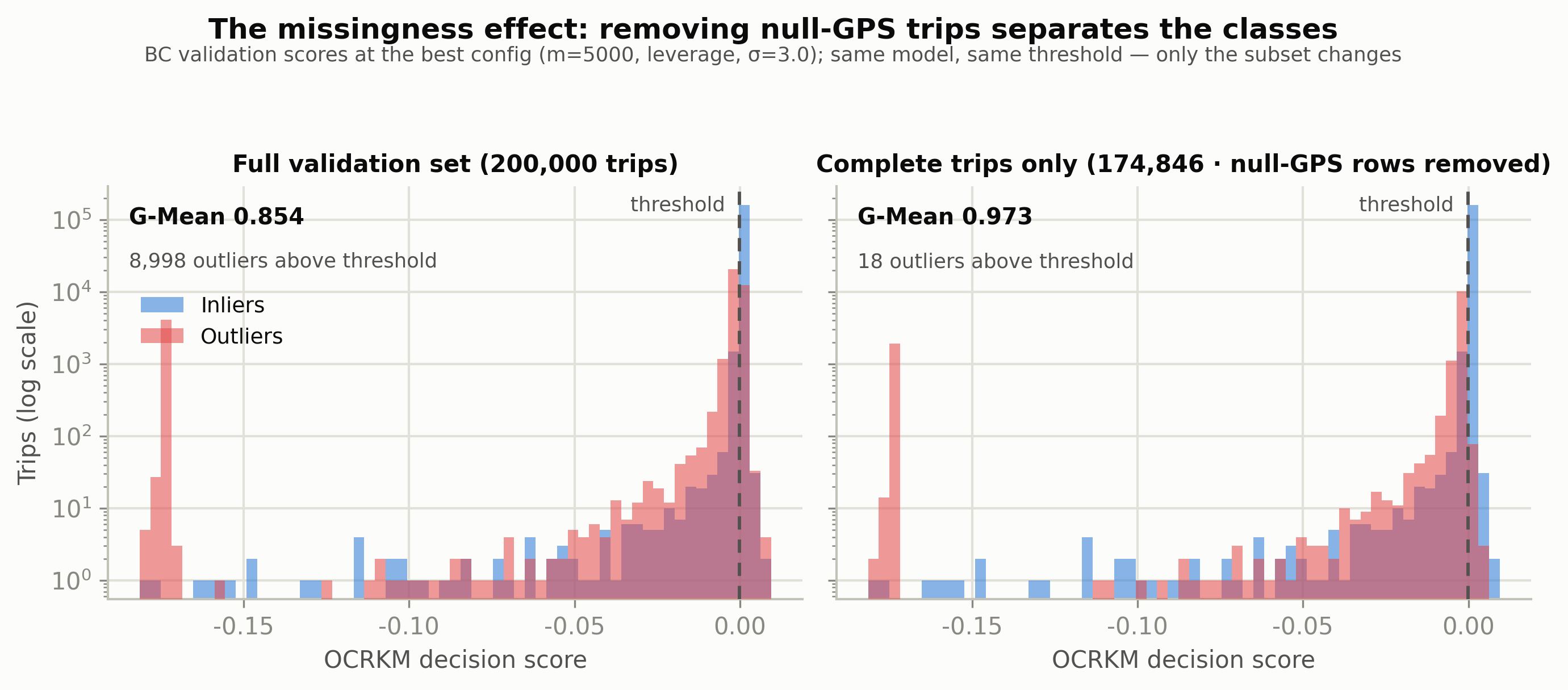
3. The “hard” dataset was hard because of missing data — and I could prove it. Trips with null GPS fields dragged aggregate G-Mean to 0.85. Restricting to complete trips — same model, same threshold — lifted it to 0.97, collapsing 8,998 missed outliers to 18. The replication then confirmed the mechanism from the opposite direction: public NYC data has no missingness, and the gap vanished.

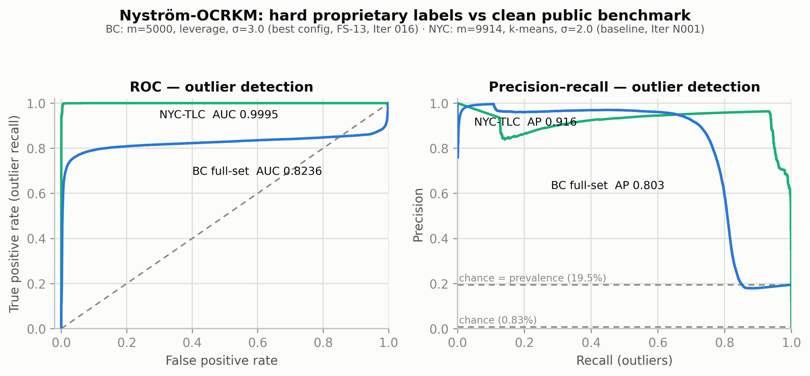
4. Clean public benchmarks understate how much these choices matter. On public NYC-TLC data — 12.3M trips censused, 18 months acquired, 6.3 GB — the task saturates: G-Mean 0.994, ROC-AUC 0.9995. At that ceiling, the landmark-strategy spread compresses from 0.10 to 0.005 and the σ effect from 0.19 to 0.002. The design choices that decide deployment performance on messy operational data are invisible on the clean benchmark. Evaluate one-class methods only on public datasets and you’ll conclude these choices don’t matter — on real data, they do.

What I’d want a reviewer to know

The baselines win on the leaderboard. On the full BC evaluation set, SGD-OCSVM (G-Mean 88.6%) and IsolationForest (87.2%, 23× faster) both beat Nyström-OCRKM’s aggregate numbers, and the paper says so. The reason to keep the kernel machine is what the aggregates hide: on a post-hoc cohort of 806 rule-compliant trips with anomalous feature combinations, IsolationForest independently confirmed all 806 — and SGD-OCSVM scored all 806 as inliers. The linear-boundary method had learned to approximate the rule system it was supposed to see past; the density-based methods learned the distribution. For a regulator whose rules already cover the easy cases, that complementary coverage is the point.

The negative results are in the paper: three engineered datetime features all hurt performance — they inflate false alarms faster than they catch new anomalies. I also reconciled a sensitivity/specificity labeling swap between the original course paper and the code’s evaluation convention (the numbers agree exactly once fixed), and cut one headline claim that traced to no artifact. The figure pipeline re-runs both models from the prepared arrays and asserts the reproduced metrics against the experiment log before it will render anything.

Stack & scale

Python (NumPy, scikit-learn, PyArrow), MLflow experiment tracking, uv environments. BC: 2M regulator records, 200k-trip validation. NYC: 12.3M-trip rule census, 18 months of parquet acquired from the Azure Open Datasets mirror (the official TLC files strip coordinates for this era), deterministic 2M sample, chunked prediction to keep peak memory at ~1.5 GB instead of ~16 GB.

The BC data is collected under a regulatory mandate and is not redistributable; the NYC-TLC replication exists so every headline claim is reproducible from public data. Full manuscript, label rules, 12.3M-trip census, and append-only experiment logs live in the project repository — public link to follow.